KEY to Exercises: Continuous Outcome, Several Independent Groups

(1) ALCOHOL.REC

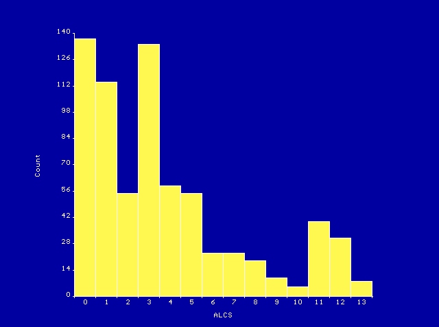
(A) Univariate. The mean alcohol consumption score is 3.7, standard deviation = 3.6, n = 713. The five-point summary: 0, 1, 3, 5, 13. Click here for the histogram. This histogram shows data to have a pronounced positive skew with modes at 1, 3, and 11.

(B) ALCS consumption by INC group

                     MEANS of ALCS for each category of INC
INC               Obs      Total       Mean   Variance    Std Dev
1                  46        130      2.826      9.791      3.129
2                  88        341      3.875     17.329      4.163
3                 140        624      4.457     17.343      4.165
4                 250        877      3.508     12.355      3.515
5                 189        672      3.556      8.642      2.940

INC           Minimum     25%ile     Median     75%ile    Maximum       Mode
1               0.000      0.000      3.000      4.000     13.000      0.000
2               0.000      0.000      3.000      5.500     13.000      0.000
3               0.000      1.000      3.000      7.000     13.000      0.000
4               0.000      1.000      3.000      5.000     13.000      0.000
5               0.000      2.000      3.000      4.000     12.000      3.000

                                     ANOVA
Variation          SS   df          MS  F statistic    p-value
Between       131.194    4      32.798        2.563   0.037300
Within       9060.127  708      12.797
Total        9191.321  712

                  Bartlett's test for homogeneity of variance
    Bartlett's chi square =  25.851  deg freedom =  4   p-value = 0.000034
         Bartlett's Test shows the variances in the samples to differ.
              Use non-parametric results below rather than ANOVA.

                  Kruskal-Wallis One Way Analysis of Variance
Kruskal-Wallis H (equivalent to Chi square) =       7.793
                         Degrees of freedom =           4
                                    p value =    0.099446

• There's evidence of unequal variance in these data. (Notice how standard deviations vary and how the Bartlett's test derives a small p value. Therefore, I conclude groups are "heteroscedastic." Group 5 shows the smallest standard deviation (s₅ = 2.9) and Groups 2 and 3 show the largest standard deviations (s₂ @ s₃ = 4.2).
• Mean alcohol scores vary from 2.8 to 4.5, with income level 3 having the highest mean score and income level 1 having the lowest. The K-W test derives p = .099 which provides weak to moderate support against the H₀ of "equal locations." Given the descriptive statistics (esp. the large difference in means), I would conclude the groups differ.

(2) DEERMICE

Summary Statistics of Weight Gain  (grams)

ANOVA results: F(2,12) = 29.69; p = .000089.

(3) ROOSTER.Testosterone by Rooster Strain

Testosterone (µg/dl)	Strain A   n = 6	Strain B  n = 6	Strain C   n = 6
Mean ± SD	43.27 ± 274.0	112.8 ± 10.5	102.0 ± 7.4
(minimum, maximum)	(134, 897)	(98, 126)	(89, 110)

In testing H₀: s²₁ = s²₂ =s²₃ we find Bartlett's Chi-square(2, N = 18) = 47.99, p < .0001. Also notice how the standard deviations estimates vary (above). Therefore, it would be foolhardy to assume equal variance among groups. The Kruskal-Wallis test is used to perform our test. We find a Kruskal-Wallis Chi-square(2, N = 18) = 12.55, p = .0019 and therefore conclude the means to vary significantly. Clearly, the testosterone level in strain A is greater than that of strain B and strain C.

(4) MAT-ROLE.REC