14.1 Distinctions. Identify which of the statements are true and which are false. The odd-numbered statements are false. The even-numbered statements are true.
14.3 Doll's ecological study of smoking and lung cancer. X = per capital cigarette consumption in 1930; Y = lung cancer morality rate per 100,000 in 1950
(A) Construct a scatterplot... below. Here's my interpretation of this plot (in cryptic note format)... form = linear, direction = positive, strength appears moderate to strong; outlier: possibly but not definitely the US.
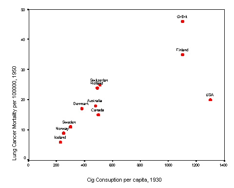
(B) Calculate the correlation coefficient... r = 0.737 @ 0.74 Interpret this statistic. This confirms the strong positive correlation.
(C) Test the correlation coefficient for significance. Show all hypothesis testing steps... H0: r = 0 versus H1: r0; tstat = (0.737 / sqrt([1 - .7372] /9)) = 3.28; df = 11 - 2 = 9; P = 0.010; conclude: the evidence against H0 is highly significant.
(D) Replicate computations in SPSS...
(E) What % of LUNGCA is "explained" by CIG? r2 = 0.54, suggesting that 54% of the variation is lung cancer mortality is [mathematically] explained by the variations in cigartette consumption.
14.5 Gravid iguanas.
(A) Construct a scatter plot of the data. Interpret your plot. linear, positive association, no apparent outlier, strong relationship.
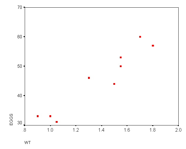
(B) Calculate the correlation coefficient. r = 0.952 (OK to use calculator software; in addition intermediate calculations shown below)
Interpret this statistic. This conforms the strong positive correlation.
[Intermediate calculations:= 1.3722l SSXX = 0.84056;
= 45.222; SSYY = 943.5516; SSXY = is 5.771 + .850 + -.056 + 4.549 + 1.383 + 5.039 + - 0.156 + 4.582 + 4.844 = 26.806; r = 26.806 / sqrt(.84056 * 943.5516) = 0.952]
(C) Test the correlation coefficient for statistical significance. H0: r = 0 versus H1: r
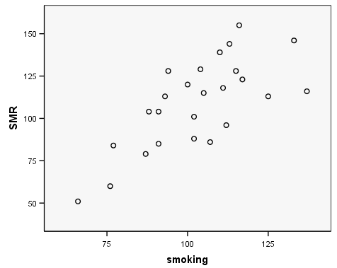
14.7. Occupational study of smoking and lung cancer.
(A) Plot the SMR against SMOKING. below Interpret the plot Form = linear, direction = positive, strength seems moderate to strong; no outliers
(B) Compute the correlation between these factors. r = 0.716 Interpret this result. This statistic confirms the strong positive association seen in the plot.
(C) Test .... H0: r = 0; tstat = 0.716 / sqrt[(1 - 0.7162) /(25 - 2)] = 4.92 with 23 df; P < 0.001, providing highly significant evidence against H0
14.9 Need and demand for mental health care. [Key not yet provided.]