15.1 Anscombe's quartet.
(A) Plot each data set ...

(B) Which data sets will support linear correlation and regression? Although all the data sets show interesting relationships, none can be adequately described by a straight line except data set 1. Linear correlation and regression are appropriate only for data set 1.
15.3 Ecological study of smoking and lung cancer.
(A) Calculate the least square regression coefficients for these data. Then show the regression model (equation) for the data.
= 6.79 + (0.0228)X
(B) Interpret the slope estimate of the model. The slope predicts 0.0228 additional cases per 100,000 person-years for each additional cigarette smoked per capita. This corresponds to an increase of 2.28 cases per 100,000 person-years for each additional 100 cigarettes smoked per capita.
(C) Predict the lung cancer mortality rate (per 100,000 person-years) in a country with annual per capita cigarette consumption of 800 cigarettes.
(D) Calculate the 95% confidence interval for the slope sY|x =([1375 - (0.0228)(32717)]/9) = 8.360; SEb = 8.360 /
(E) SPSS results...
15.5 Gravid iguanas.
(A) Calculate least squares regression estimates a and b.
(B) H0: b = 0 versus H0: b0; t stat is used: seb = 3.883; tstat = 31.89 / 3.883 = 8.21; df = 9 - 2 = 7, P
0; highly significant.
(C) What is the predicted number of eggs for a 1.2 kg iguana?
15.7 Water fluoridation and
dental cavities.
(A) Data
(B) Untransformed data 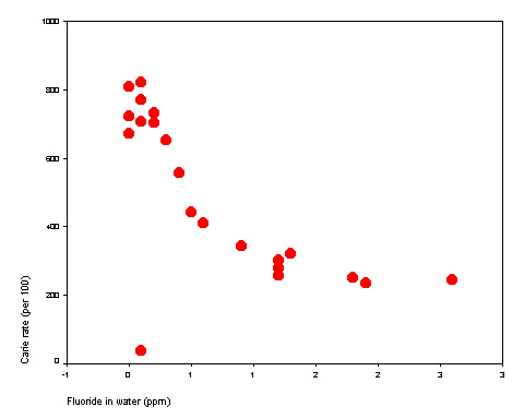 |
Interpretation:
Any outliers? Yes. Lower left quadrant -- a city with low fluoride and
low cavity rate. (Observation 21 with coordinates
0.1, 37) Relation linear? No! [Curvilinear, yes.] Relation? The scatter plot reveals an strong curved negative relation between fluoride levels and cavity rates. The steepest decline occurs between 0 and 1 ppm of fluoride. The decline levels off after this point. Unmodified linear regression would not be warranted under these circumstances (two reasons -- non-linearity and outlier). |
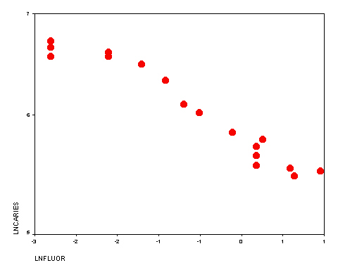
| (C) Outlier removed + ln-ln transformated
data
|
Interpretation:
Relation linear? Yes. This relation can be described by a straight line. Correlation statistics: Regression equation:
|
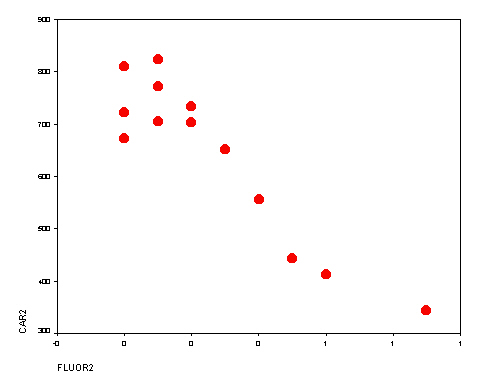
| (D) Outlier removed + range restricted
|
Interpretation: Relation linear? Not perfectly, but good enough for descriptive purposes. Correlation statistics: . Regression model: Comment: Although the fit of this model is not as good as model B, I prefer no model. The untransformed figure shows most clearly that the decline in cavity rates is steep in the 0 to 0.8 range. Since higher levels have only modest increases in benefit and potential toxicity, any action should be devoted to adding less than 1 ppm of fluoride to public water sources. |