| Background | Scatter Plot | Correlation Coefficient | Regression Model | Importance of Visualization | Exercises
In preceding chapter we considered the relation between a continuous dependent variable (Y) and categorical independent variable (X) using ANOVA. In this chapter we consider the relation between two continuous variables X and Y using correlation and regression.
Although correlation and regression are used for similar purposes, some distinctions exist. Correlation quantifies the relation between variable X and variable Y with a unit-free correlation coefficient. Regression, on the other hand, quantifies the relation between X and Y by predicting the average change in Y per unit X. Therefore, the choice of whether we use regression or correlation depends on the questions we ask of the data When the researcher wants to measure the relation between X and Y in unit-free terms, correlation is used.
Other distinctions between correlation and regression exist. A sample may be selected so that the distribution of independent variable X is fixed by the researcher or so that it is left free to vary. For example, in a study of age and blood pressure, a researcher may select a fixed number of people from various age categories (e.g., five 40-year-olds, five 50-year-olds, and so on), thus fixing the distribution of X. This is called fixed-effects or Model I sampling. In contrast, the study may sample people at random, determining their age after they are selected. This is called a random-effects model or Model II. Regression can be used with fixed-effects sampling and random-effects sampling. Correlation should be used only with random-effects sampling.
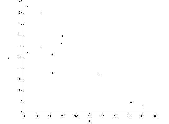
Illustrative Data. The data set BICYCLE.REC in BICYCLE.ZIP is used to illustrate correlation and regression. Data come from a study examining bicycle helmets use in 12 northern California neighborhoods. Bicycle helmet use is measured as the percentage of neighborhood bicycle riders wearing helmets (Y). Socioeconomic status is measured as the percentage of children receiving free- or reduced-fee meals at school (X). Data are:
REC SCHOOL$ X Y
--- ------------- ---------- ----------
1 Fair Oaks 50 22.1
2 Strandwood 11 35.9
3 Walnut Acres 2 57.9
4 Discov. Bay 19 22.2
5 Belshaw 26 42.4
6 Kennedy 73 5.8
7 Cassell 81 3.6
8 Miner 51 21.4
9 Sedgewick 11 55.2
10 Sakamoto 2 33.3
11 Toyon 19 32.4
12 Lietz 25 38.4
The first step in the analysis should be to plot the data in the form of a scatter plot. To draw a scatter plot with Epi Info, first READ the data set into the current session and then issue the command:
EPI6> SCATTER <X> <Y>
where <X> represents the name of the independent variable and <Y> represents the name of the dependent variable. For example, to draw a scatter plot for the illustrative data, the following commands are issued:
EPI6> READ BICYCLE
EPI6> SCATTER X Y
Click here to display the scatter plot produced by Epi Info. An inverse correlation is evident.
Comment: Observations that do not fit the general data pattern of the data are called outliers. Identifying and dealing with outliers is an important although often misunderstood statistical undertaking. In some instances, outliers should be excluded, while in others they should remain with the data. When a researcher chooses to leave the outlier in the analysis, it should be carefully scrutinized -- often, there is something to learned from the outlier. For insights into how to deal with outliers, please click: www.tufts.edu/~gdallal/out.htm (Kruskal, 1960).
Pearson's product-moment correlation coefficient (r) quantifies the relation between X and Y in unit-free terms. When r @ 0, there is no linear correlation between X and Y. When all points fall on a straight line with an upward slope, r = +1. When all points fall on a straight line with a downward slope, r = -1.
The correlation coefficient is calculated with the command issued as follows:
EPI6> REGRESS <Y> <X>
where <X> is the name of the independent variable and <Y> is the name of the dependent variable. Notice that the order of <X> and <Y> in the REGRESS command is opposite that of the SCATTER command!
For the illustrative data output is:
Correlation coefficient: r = -0.85
r^2= 0.72
95% confidence limits: -0.96 < R < -0.54
Notes:
(1) The above output shows r = -.85, showing a strong negative correlation between X and Y.
(2) The 95% confidence interval locates correlation coefficient parameter r with 95% confidence. Report this as "95% confidence interval for r is (-0.96, -0.54).
(3) The statistic labeled r^2 is the coefficient of determination. This represents the proportion of the variance in one variable explained by the other. The illustrative example demonstrates a coefficient of determination of 0.72, suggesting 72% of the variance in helmet use is explained by socioeconomic status.
Regression models predicts the value of Y for a given value of X according to the equation:
Y = (INTERCEPT) + (SLOPE)X + (RANDOM ERROR)
In recognizing the above equation as that of a line, the INTERCEPT identifies where the line crosses the Y axis and SLOPE represents the line's include or "change in Y per unit X." The RANDOM ERROR term allows for statistical scatter around the line and is assumed to be normally distributed with a mean of 0 and variance of s2. Thus, regression equation describes a line that travels through the scatter cloud while accounting for random error in the data.
So how does one calculate the line's slope and intercept? The method we uses minimizes the sum of the RANDOM ERROR values around the line and is thus called the least squares line.
The least square line is calculated by the REGRESS command with coefficients reported as follows:
B 95% confidence Partial
Variable Mean coefficient Lower Upper Std Error F-test
X 30.8333 -0.5386091 -0.746144 -0.331074 0.105885 25.8748
Y-Intercept 47.4904464
The B coefficient for X is the slope of the model. This predicts the average change in Y per unit X. For the illustrative example
the slope of -0.54 predicts a 0.54 decrease in Y with that each unit of X.
(2) The B coefficient for the Y-intercept for this model is 47.4904. Therefore, the regression model is: Y = 47.49 +
(-0.54)xi + (RANDOM ERROR).
Notes:
(1) This equation can be used to predict helmet use rates in various communities. For example, a neighborhood in which half the children receive free- lunches (i.e., X = 50), Y = 47.49 + (-0.54)(50) = 20.5.
(2) A 95% confidence interval for b1 is provided by the REGRESS command. For the illustrative example, the 95% CI for b1 = (-0.746, -0.331).
Exploration of scatter plots can prevent the reporting of nonsensical results. The data sets known as Anscombe's Quartet:
| Data Set I | Data Set II | Data Set III | Data Set IV | ||||
| X | Y | X | Y | X | Y | X | Y |
| 10.0 8.0 13.0 9.0 11.0 14.0 6.0 4.0 12.0 7.0 5.0 |
8.04 6.95 7.58 8.81 8.33 9.96 7.24 4.26 10.84 4.82 5.68 |
10.0 8.0 13.0 9.0 11.0 14.0 6.0 4.0 12.0 7.0 5.0 |
9.14 8.14 8.74 8.77 9.26 8.10 6.13 3.10 9.13 7.26 4.74 |
10.0 8.0 13.0 9.0 11.0 14.0 6.0 4.0 12.0 7.0 5.0 |
7.46 6.77 12.74 7.11 7.81 8.84 6.08 5.39 8.15 6.42 5.73 |
8.0 8.0 8.0 8.0 8.0 8.0 8.0 19.0 8.0 8.0 8.0 |
6.58 5.76 7.71 8.84 8.47 7.04 5.25 12.50 5.56 7.91 6.89 |
Identical correlation and regression statistics are derived for each of these data set (INTERCEPT = 3, SLOPE = 0.5, r = +0.82, etc.). However, scatter plots reveal distinct relations (Fig.). Data set I demonstrates scatter typical of a statistical positive linear relation. Data set II a complex nonlinear curve. Data set II demonstrates a perfect linear relation with one outlier. Data set IV demonstrates no variability in X with the exception of an outlier in the upper right quadrant.
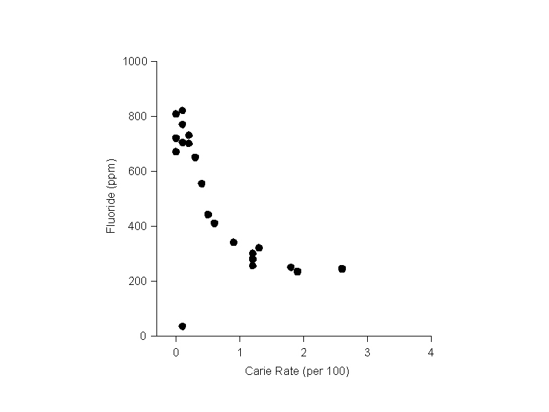
Another example is provided by the data in WATER.ZIP (Dean, 1942). Data in this file are from a study on water fluoridation. and cavity rates. The variables are FLUORIDE (parts per million) and CARIES (dental caries per 100 children). A scatter plot of the data (click here) reveals an decline in cavity rates as fluoride levels up to 1 ppm. There is an outlier in the lower left quadrant (record 21). Although unmodified regression should not be applied to this pattern, we still have the following options:
The last option is achieved by issuing the command SELECT FLUORIDE <= 1 before issuing the REGRESS CARIES FLUORIDE command. This derives the following output:
Correlation coefficient: r = -0.92
r^2= 0.86
95% confidence limits: -0.98 < R < -0.76
Source df Sum of Squares Mean Square F-statistic
Regression 1 248393.9485 248393.9485 65.13
Residuals 11 41950.3592 3813.6690
Total 12 290344.3077
B Coefficients
B 95% confidence Partial
Variable Mean coefficient Lower Upper Std Error F-test
FLUORIDE 0.2615 -528.0656304 -656.311967 -399.81929 65.431804 65.1325
Y-Intercept 780.3402418
The slope of -528 suggests that one ppm of fluoride is associated with an expected reduction of 528 cavities per 100 children in the range 0 - 1 ppm. Assuming linearity, this is equivalent to -52.8 per 100 children for each 0.1 ppm of fluoride. The coefficient of determination (r2) of 0.86 suggests that 86% of the variance in carie rates in this range is explained by fluoride level.
(1) BIGTEN.ZIP. Graduation Rates at Big Ten Universities (Data from Berk, 1994, p. 82). Download and unzip the data set BIGTEN and then explore the relation between five-year graduation rates (UPERCENT) and the scores of incoming freshman on the ACT exam (ACT).
(2) IGUANA.ZIP. Iguana Eggs Over Easy (Data from Hampton, 1994, p. 157). Listed below are data representing the body weight and number of eggs produced by 9 gravid female iguanas. Analyze the data using both correlation and regression techniques. Remember to interpret your findings.
ID Weight Eggs
--- ------ ------
1 0.90 33
2 1.55 50
3 1.30 46
4 1.00 33
5 1.55 53
6 1.80 57
7 1.50 44
8 1.05 31
9 1.70 60
(3) ALCOHOL.ZIP. Alcohol Consumption Survey (Data from Monder, 1986). Download and unzip the data set ALCOHOL.REC (used in the previous chapter) and determine the linear relation between alcohol consumption (ALCS) and AGE using correlation and regression techniques. Because the scatter plot is difficult to interpretable, assume any relation will be linear, without outliers, and meet other regression assumptions.
Ansombe, F. J. (1973). Graphs in statistical analysis. American Statistician, 27, 17-21.
Berk K. N. (1994). Data Analysis with Student SYSTAT. Cambridge, MA: Course Technology.
Dean, H. T. (1942). Arnold, F. A., & Elvov, E.. Domestic water and dental caries. Public Health Reports, 57, 1155-1179.
Hampton, R. E. (1994). Introductory Biological Statistics. Deburque, IW: Wm. C. Brown.
Kruskal, W. H. (1960) Some remarks on wild observations. Technometrics Available: www.tufts.edu/~gdallal/out.htm.
Monder, H. (1986). [Alcohol consumption survey.]. Unpublished data.
Perales, D. & Gerstman, B. B. A bi-county comparative study of bicycle helmet knowledge and use by California elementary school children. The Ninth Annual California Conference on Childhood Injury Control, San Diego, CA, March 27-29, 1995.