Background | Indicator Variables | Multiple Regression Model | Exercises | Appendix
The prior chapter used simple linear regression to describe the relation between a single independent variable X and dependent variable Y. In this chapter, we use multiple linear regression to describe the relation between multiple independent variables X1, X2, ... , Xk and dependent variable Y.
Recall that the simple regression model is:
yi = b0 + b1xi + ei
where b0 represents the intercept coefficient, b1 represents the slope coefficient, and ei represents the residual error term. Multiple regression extends this model to include multiple independent variables:
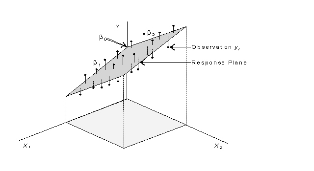
yi = b0 + b1x1i + b2x2i + ...+ bkxki + ei
Just as a simple regression model constructs a regression line in two-dimensional space, multiple a regression model with two independent variable constructs a regression plane in three-dimensional space [Fig.]. When considering k independent variables, the multiple regression model fits a regression plane in k + 1 dimensional space. Although we cannot visualize placed beyond three-dimensional space, linear algebra allows their expression numerically.
Illustrative Data Set. We use the data set FEV.REC to demonstrate techniques in this chapter. Data are part of a respiratory health survey in children and adolescents. There are 654 observations in our data set. The dependent variable for our illustrations is forced expiratory volume (FEV). This is a measure of pulmonary function, determined as the peak air flow measured in liters per second. For our illustration we are interested in measuring the effects of smoking (SMOKE coded 1 = current smokers, 0 = non-smoker) and AGE (years) of FEV.
Notice that the variable SMOKE is binary ("dichotomous"). Regression models can accommodate dichotomous independent variables by coding them 0 to indicate absence of the attribute and 1 to indicate presence. A binary variable coded in this way, which may be referred to as an indicator variable, dummy variable, or zero/one variable, may be included in regression models like any other variable. For example, to analyze the effects SMOKE on FEV, issue the commands,:
EPI6> READ FEV
EPI6> REGRESS FEV SMOKE
Output is:
ß 95% confidence Partial
Variable Mean coefficient Lower Upper Std Error F-test
SMOKE 0.0994 0.7107189 0.495231 0.926206 0.109943 41.7892
Y-Intercept 2.5661426
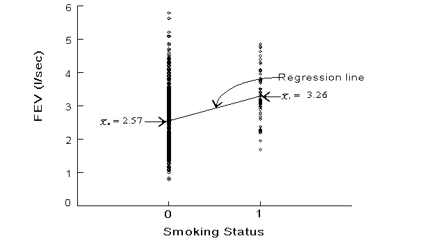
The slope coefficient of 0.71
for SMOKE and FEV suggests hat FEV increases 0.71 units
(on the average) as we go from SMOKE = 0 (non-smoker) to SMOKE = 1 (smoker) (Fig.). This slope
corresponds to the sample mean difference (![]() 0
-
0
-
![]() 1).
Moreover, the confidence interval for the slope corresponds to a confidence interval for �0 - �1.
In summary, the mean difference in FEV in smokers and non-smokers is 0.71 (95% confidence interval:
0.50, 0.93). This is surprisingly given what we know about smoking.
How can a
positive relation between SMOKE and FEV
exist given
what we know about the physiological effects of smoking? The answer lies in
understanding the confounding effects of AGE on SMOKE and FEV. In this
child and adolescent population, nonsmokers are
younger than nonsmokers (mean ages: 9.5 years vs. 13.5 years, respectively). It is
therefore not surprising that AGE confounds the relation
between SMOKE and FEV. So what are we to do?
1).
Moreover, the confidence interval for the slope corresponds to a confidence interval for �0 - �1.
In summary, the mean difference in FEV in smokers and non-smokers is 0.71 (95% confidence interval:
0.50, 0.93). This is surprisingly given what we know about smoking.
How can a
positive relation between SMOKE and FEV
exist given
what we know about the physiological effects of smoking? The answer lies in
understanding the confounding effects of AGE on SMOKE and FEV. In this
child and adolescent population, nonsmokers are
younger than nonsmokers (mean ages: 9.5 years vs. 13.5 years, respectively). It is
therefore not surprising that AGE confounds the relation
between SMOKE and FEV. So what are we to do?
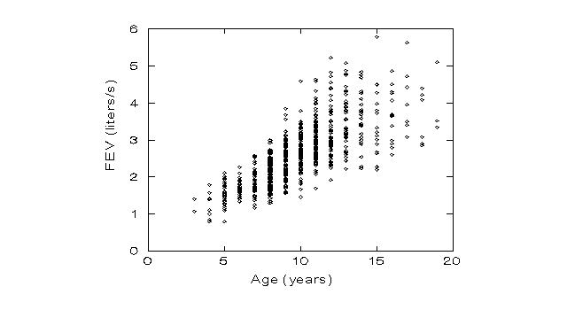
Confounding is a bias due to non-comparability of groups. For the current example smokers are older than nonsmokers, and age is a strong predictor of the outcome (Fig.). Therefore, the relation between FEV and SMOKE is confounded by AGE. Fortunately, we can use multiple regression to adjust for this problem. In effect, multiple regression will balancing the effects of age at all levels as we compare smokers and non-smokers.
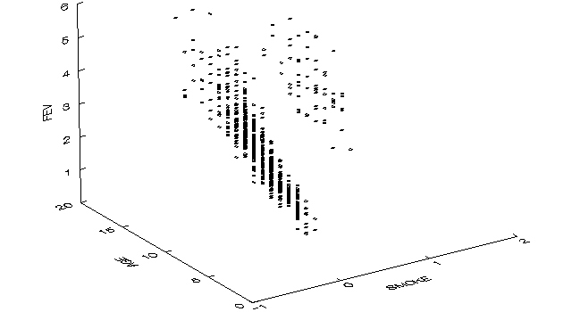
Imagine we hold AGE constant while describing the relation between SMOKE and FEV. This can be visualized with a three-dimensional scatter plot with separate scatter clouds for nonsmokers and smokers (Fig.). The question now becomes "Which scatter cloud is higher?" I suggest the nonsmokers cloud is higher all along the cloud.
To have Epi Info calculate multiple regression coefficients issue the command:
EPI6> REGRESS <Y> <X1> <X2>
For the current illustrative data issue the command:
EPI6> REGRESS FEV SMOKE AGE
Output is:
b 95% confidence Partial
Variable Mean coefficient Lower Upper Std Error F-test
SMOKE 0.0994 -0.2089949 -0.367256 -0.050734 0.080745 6.6994
AGE 9.9312
0.2306046 0.214563 0.246646 0.008184 793.8988
Y-Intercept 0.3673730
We now have separate regression
coefficient for the independent variables. Thus, the model is:
FEV = 0.37 + (-0.21)(SMOKE) + (0.23)(AGE)
The researcher interprets each adjusted slope with less concern for confounding. In this instance the regression coefficient for SMOKE shows a negative relation with FEV (smoking decreases FEV by .21 units).
As was the case with simple regression, the multiple regression model can be used to predict the average FEV value for a given observation. For example, the average non-smoking (SMOKE = 0), 10-year old (AGE = 10) is predicted to have FEV = 0.37 + (0.21)(0) + (0.23)(10) = 2.67.
95% confidence intervals are provided for each slope parameter. For the illustrative example, the 95% confidence interval for bSMOKE is (-0.37, -0.05) and the 95% confidence interval for bAGE is (0.21, 0.25).
Assumptions. The "LINE" assumptions (Linearity, Independence, Normality, and Equal variance) required by simple linear regression are no less important in multiple regression that they are in simple linear regression. They are more difficult to evaluate, however. Some computer programs are equipped with graphical diagnostics for this purposes. Epi Info, however, has no such facilities. At the very least, scatter plots of bivariate relations (e.g., Y vs. X1, Y vs. X2, and so on) should be explored for linearity.
(1) BIGTEN.ZIP. Graduation Rates at Big Ten Universities (Berk, 1994, p. 82). In a previous exercise we found a strong positive relation between university graduation rates (UPERCENT) and the average ACT score of incoming freshman (b = 5.4, 95% confidence interval for b= 3.1 - 7.8). However, other factors such as freshman class size may also exert influence on graduation rates. Include the variable FRESH (freshman class size) in your model describing the relation between UPERCENT and ACT. Report your findings.
(2) ALCOHOL.ZIP: Alcohol Consumption Survey (Monder, 1986). Recall the ALCOHOL.REC data set introduced in a previous chapters. Previously we had found that alcohol scores (ALCS) were inversely related with AGE. The relation between ALCS and INCome formed a U-shape (lowest alcohols score average in the middle income group). We now want to run a multiple regression analysis in which the independent contribution of both AGE and INC are evaluated.. (To do this, you will have to convert INC is into 4 separate dummy variables.) Present a multiple regression model for these data.
(3) MPT.ZIP. Math Pre-Test Scores and Performance on a Biostatistics Test. A math test is given to students coming into a biostatistics class. Data from the math pretest (MPT) , the students' major (MAJORX: 1 = major X, 0 = other major), and scores from exam 2 (EX2) are stored in MPT.REC. Describe the independent contributions of MPT and MAJORX on EX2.
Categorical variables with k categories (k > 2) can be made into indicator variables by turning them into k - 1 indicator variables. For example, a categorical variable with values A, B, and C can be re-coded into two indicator variables (DUMMY1 and DUMMY2) as follows:
EPI6> IF X = "A" THEN DUMMY1 = 1 ELSE DUMMY1 = 0
EPI6> IF X = "B" THEN DUMMY2 = 1 ELSE DUMMY2 = 0
Data are transformed as follows:
| Original Value of X | Value of DUMMY1 | Value of DUMMY2 |
| A | 1 | 0 |
| B | 0 | 1 |
| C | 0 | 0 |
Given the many possible factors that might influence an outcome, one of the greatest challenges of multiple regression is the selection of variables that will comprise the model. Although an extensive review of this problem is beyond the scope of this brief presentation, a few words of introduction seem appropriate. Variable selection strategies depends on the ultimate use of the model. Statistical analyses, in general, have three major uses. These are: (1) description, (2) prediction, and (3) control. The dominant concern of most epidemiologic studies is describing the unbiased relation between a independent variable X1 and the dependent variable Y with variables other than X1 considered as potential confounders. The goal, then, is to seek a parsimonious model (the model with the fewest covariates) that accurately reflect the causal relation between X1 and Y relation. To accomplish this goal, we start by considering all known risk factors for Y. A lengthy list of variables is created. The analyst then narrows down the list to include only those factors deemed relevant to the the X1/Y relation. The analysts should NOT let the computer select variables based on any "forward" or "backward" algorithm.