15: Regression 3/14/07

Review Questions

1. How does regression differ from correlation?
2. How does an algebraic line differ from a statistical line?
3. Lines are characterized by their slope and intercept. What does the slope tell you about the line? What does the intercept tell you?
4. What does a slope of 0 indicate?
5. What is "squared" in a least squared regression line?
6. Suppose the relation between AGE (years) and HEIGHT (inches) in an adolescent population is described by this model: = 46 + 1.5X. Interpret the slope of this model. Then, predicted the average height of a 10 year-old.
7. What t value do you use when calculating a 95% confidence interval for b when n = 25? 
8. What symbol is used to denote the slope in the data? What symbol is used to denote the slope in the population?
9. Under the null hypothesis, beta = ______. 
10. Negative slopes suggest that as X increases, Y tends to _______________.
11. The Normality and equal variance assumptions for regression refer to the distribution of the _____________.
12. What is confounding?
13. What is a residual? 
14. What distributional conditions are necessary to help infer population slope beta? 
15. Vocabulary: least squares method, regression coefficients, slope estimate (b), slope parameter  (b), intercept estimate (a), intercept parameter (a), ("y hat"), standard error of the regression (s_Y|x), standard error of the slope (SE_b).

Exercises

15.1  Anscombe's quartet. Graphs are essential to good statistical analysis, so begins the often cited article by Anscombe (1973; link to full text). This exercise demonstrates why it is important to look at a graph of the data before conducting numerical analyses. Data for four bivariate data sets are shown below and are stored online in anscomb.sav. Each data sets is characterized by these same numerical results: n = 11, = 9.0, = 7.5, r = 0.82, = 3 + 0.5X, and P = 0.0022. 

(A) Plot each data set on four separate graphs. You are encouraged to use SPSS or other software to complete your plots. If you wish to plot the points by hand, please use graph paper. If you are pressed for time, you may merely look at the plots in the key.
(B) Which of these data sets will support linear correlation and regression? Explain your response.

15.2 Farr�s study of elevation and cholera mortality. William Farr (1807�1883) is a titan in the history of epidemiology and public health. He was the first Registrar General of a national vital statistics organization and he innovated many of the methods still used today to collect and analyze population-based health statistics. At the same time, like many of his contemporaries, Farr erroneously believed that epidemics were caused by spontaneous generations and miasmas (bad air) that emanated from the environment; Farr was not a contagionist. In 1852, Farr reported on the association between low elevation and cholera. Some of his data are reported below. Data are stored online in ../datasets/farr1852.sav.

(A) What is the independent variable in this analysis? What is the response variable?
(B) Create a scatterplot of the data. Describe the relation (form, direction, strength, outliers) between elevation and cholera mortality. Is the relation linear? 
(C) Mathematically transform the data to a natural logarithmic scale. Plot the transformed data point. Describe the relationship of the transformed data.
(D) Farr used these data to support the theory that bad air had settled into low-lying areas causing outbreaks of cholera. We now know that air quality has nothing to do with causing cholera . In fact, the water-borne bacterial Vibrio cholera causes the disease. Suggest confounding variables that may have explained the strong association between elevation and cholera mortality. 

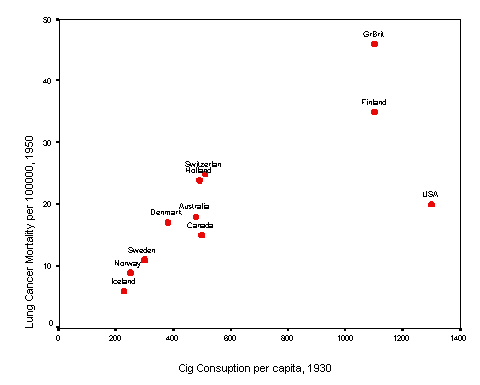
15.3 Ecological study smoking and lung cancer . These Exercises is an extension of Exercise 14.3. Recall that X = regional per capita 1-year cigarette consumption in 1930 and Y = lung cancer mortality (per 100,000 person-years) 20 years later. The scatter plot revealed a linear positive association. Although the data point for the U.S. was lower than expected, we could not say with certainty whether it was an outlier. Overall, r = 0.74 (P = 0.010).

(A) Calculate the least square regression coefficients for these data. Then show the regression model (equation) for the data.
(B) Interpret the slope estimate of the model. 
(C) Predict the lung cancer mortality rate (per 100,000 person-years) in a country with annual per capita cigarette consumption of 800 cigarettes.
(D) Calculate the 95% confidence interval for the slope. Interpret this interval.
(E) Replicate the regression analysis in SPSS. The data set is stored online as  doll-ecol.sav. Menu choices for linear regression are Analyze > Regression > Linear. After running the program, identify the following statistics in the output: r,  r² and the P value for testing H₀: b = 0. Also find the intercept coefficient (reported as the "unstandardized (Constant) coefficient") and slope coefficient (reported as the unstandardized coefficient for the independent variable). Coefficient may be reported in scientific notation. For example, 2.284E-02 means 2.284 � 10^-2 = 0.00284. 

15.4 Sodium consumption and blood pressure. Recall Ex. 14.4 in which X = sodium intake (g/day) and Y = systolic blood pressure (mm Hg). We found n = 10, SS_XX = 0.409, SS_YY = 1979.600, SS_XY = 26.18,  = 7.11, = 174.2, and r = 0.92. Click here for the scatter plot.

(A) Determine the regression model for these data. Show all work. Write down the regression equation for these data. Interpret the slope and intercept of your regression model. 
(B) Predict the systolic blood pressure of a person from this population with a salt intake of 7.2 g/day.
(C) Calculate the standard error of the regression and the standard error of the slope.
(D) Calculate the 95% confidence interval for the slope. Interpret your results.
(E) Data are available in na-bp.sav. Download the data set and replicate your analyses in SPSS in order to check your results.

15.5  Gravid iguana. Recall the Exercise 14.4 concerning the analysis of gravidity and iguana body weight. From this prior exercise, we learned there was a strong positive linear relation between body weight and number of eggs produced: r = 0.952 (P = 0.000076). Statistics included: n = 9, = 1.3722, SS_XX = 0.84056, = 45.222, SS_YY = 943.5516, and SS_XY = 26.806.

(A) Calculate least squares regression estimates a and b. Interpret the slope coefficient. How much would a 0.1 kg. increase in body weight increase eggs production.
(B) Test H₀: b = 0. Show all testing steps. 
(C) What is the predicted number of eggs for a 1.2 kg iguana?
(D) Replicate the above analyses with SPSS. If you find a discrepancy between your hand calculations and those produced of SPSS, track down your  your error and correct it.

15.6 Graduation rates @ Big Ten universities. Exercise 14.6 introduced this data set. Recall that this data set looked at average ACT scores of incoming freshman as a predictor of the percent of university students graduating within 5 years  (UPERCENT). Here are summary statistics for these data: n = 7, = 24.429, SS_XX = 29.714, = 63.971, SS_YY = 1090.374, SS_XY = 161.886, and r = 0.90.

(A) Determine the least square regression line for these data. 
(B) Interpret the slope of the model.
(C) Test H₀: b = 0. Show work. 
(D) Based on your model, what is the predicted graduation rate for a class with an average ACT of 25?

15.7 Water fluoridation and cavity rates. Data are from a study of 7,257 children in 21 cities. The explanatory variable is FLUORIDE level in public water supplies (parts per million). The response variable is CARIES (the number of cavities per 100 children) . Data are stored in water.sav and are listed below (Pagano & Gauvreau, 1993, p. 377 - 378; Dean et al., 1942 with an intentional data entry error). 

OBS  FLUORIDE  CARIES
 1    1.9      236
 2    2.6      246
 3    1.8      252
 4    1.2      258
 5    1.2      281
 6    1.2      303
 7    1.3      323
 8    0.9      343
 9    0.6      412
10    0.5      444
11    0.4      556
12    0.3      652
13    0.0      673
14    0.2      703
15    0.1      706
16    0.0      722
17    0.2      733
18    0.1      772
19    0.0      810
20    0.1      823
21    0.1       37

(A) Download water.sav or enter it into your statistical package. 
(B) Construct a scatterplot of the data (Graph > Scatter). Describe what you see. Are there any outliers? Is this relation linear? If the relation is not linear, what type of relation do you see? Would unmodified linear regression be warranted under these circumstances?
(C) Although unmodified regression does not apply to these data, we may still build a valid model using one of a number of methods. One method is to exclude the outlier and straighten-out the relation with algebraic transforms. As an example, we will apply a logarithmic transforms to both the FLUORIDE variable and the CARIES variable. 

• Make a copy of the data file. Call the new file water2.sav.Open water2.sav in SPSS. 
• Find the outlier in the data table (observation 21). Delete this observation.

• From the main SPSS menu, click Transform > Compute. A dialogue box will appear. Fill in the Target Variable field with the  new variable name lncaries and fill the Numeric Expression field with ln(CARIES). Click OK. A new column appears in the Data View containing a logarithmic transform of the CARIES variable.

• Perform a logarithmic transform on the FLUORIDE variable. 
• Plot the ln-ln transformed data. Is the relation linear? 
• Run a regression analysis on transformed data. Write down the regression equation and interpret your model.

(D) Another way to analyze these data is to eliminate the outlier and then restrict the analysis to a range that can reasonably be described with a straight line. 

• Open water2.sav (if it is not already opened).
• Cut and paste the original data into two empty columns. Call these new variables FLUOR2 and CAR2, respectively. 
• Sort the data on FLUOR2. (Data > Sort Case -- select FLUOR2 > OK.) 
• In the FLUOR2 and CAR2 columns, delete cases with FLUOR2 values greater than 1 ppm. 
• Plot FLUOR2 and CAR2 as a scatter plot. Discuss the plot.
• Run a regression analysis on FLUOR2 and CAR2. Report and interpret all relevant statistics.

15.8 Maternal mortality and health care during birth. Recall Ex 14.8 in which the relation between the percentage of births attended by health care professionals (ATTENDED) and maternal mortality (MAT_MORT) were recorded for 11 countries. The strong negative association between these factors was shown to be linear. Descriptive and correlation statistics for these data are:

(A) Calculate the least squares regression coefficients for these data. Report the regression model, and interpret its slope.
(B) What is the predicted maternal mortality rate in a country that has 80 percent of births attended by professionals?
(C) Calculate a 95% confidence interval for b. 

Key to Odd Numbered Problems                                  Key to Even Numbered Problems (may not be posted)